Month: September 2025

Continuing our hypothetical study of how high school coaches (specifically football coaches) can implement data technologies and use them to help save time and focus on coaching and developing players and students.

You’ve got the Saturday grading workflow dialed in (position tabs, per‑player per‑play grades, simple notes, and a Monday “Team Sheet”). Now let’s zoom out: how do you turn that weekly rhythm into cumulative insight—tracking every kid’s growth across the season (and across seasons), spotting unit‑level trends, and making November decisions with March‑level clarity? The short answer: pair your staff’s grading discipline with a data engineer who stands up a light, durable analytics stack in Microsoft Fabric and Power BI. Fabric gives you one place to land, shape, secure, and publish your data—end‑to‑end—without stitching together a dozen services.

Below is a coach‑first, high‑level guide to “what we’ll do” and “who does what,” building directly on the grading app/process described in the post you just read.

The Coach–Data Engineer Playbook

Coaches (what you already do):

• Grade each snap with the simple rubric (+ / 0 / – / ME) and one‑phrase notes where they matter.
• Tag a handful of teaching reps.
• Keep the grading standards consistent so the data stays trustworthy.

Data Engineer (what they add):

• Wire up a single, durable data lake and semantic model so Saturday’s grades automatically become Monday’s dashboards—and season trends.
• Ensure privacy (players only see their data), reliability (no “did it refresh?” panic), and speed (reports open instantly).
• Set and enforce definitions so “Grade %,” “ME rate,” and “Explosive” mean the same thing in October as they did in Week 1.

The season‑long architecture (in plain language)

Think of this as three layers—Operate → Store/Shape → Show—with governance wrapped around everything.

1) Operate (your grading apps)

• You’re already capturing Players, Games, Plays, On‑Field, Grades in Power Platform (Dataverse). That’s your operational system.

Data engineer’s move: Turn on Link to Microsoft Fabric from Dataverse so your tables are automatically and efficiently mirrored into OneLake (Fabric’s single, organization‑wide data lake) as Delta tables—made for analytics. No export jobs to babysit.

Why this matters: OneLake gives you “one copy” of your data that every analytics engine in Fabric and Power BI can use—faster, cheaper, and simpler than duplicating data all over the place.

2) Store & Shape (the lakehouse)

Inside Fabric, the engineer sets up a Lakehouse with a simple “medallion” flow:

• Bronze: the raw mirrored tables from Dataverse (unchanged).
• Silver: cleaned, typed, coach‑friendly columns (e.g., standardized grade codes, consistent position groups).
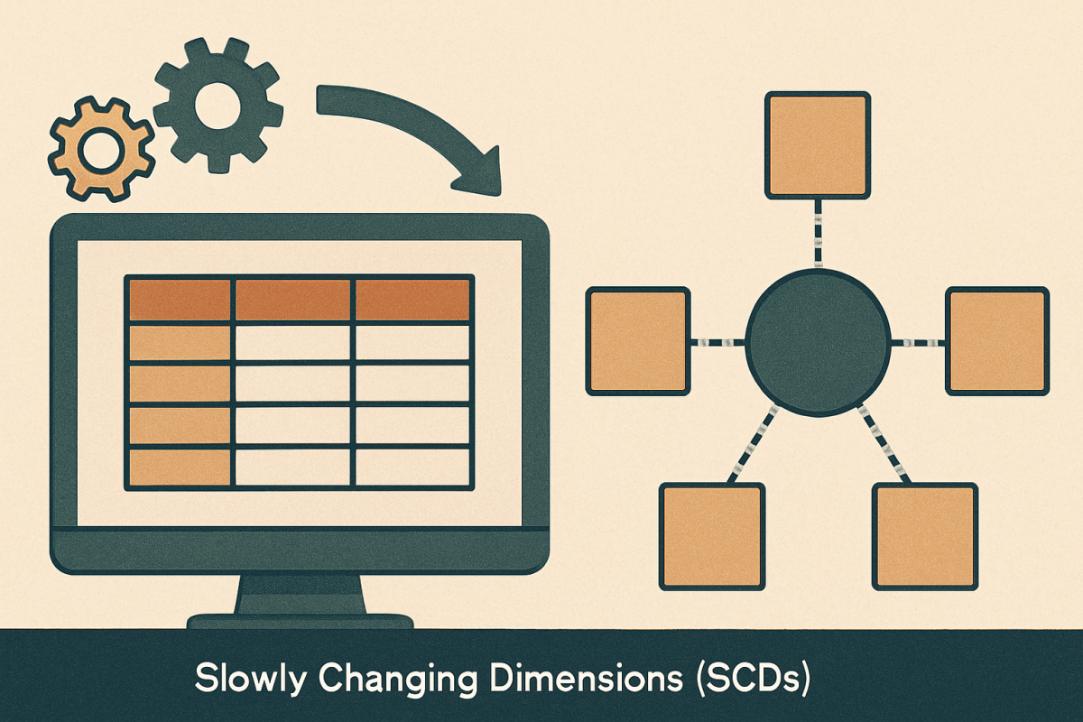
• Gold: a star schema built for analysis:
  • Dimensions: DimPlayer, DimGame, DimOpponent, DimPositionGroup, DimUnit.
  • Facts: FactPlayerPlayGrade (one row per player‑play), FactPlayerGame (rollups), and optional FactEvent(penalties, explosives, pressures).

Need to bring in other data (attendance, GPS, a scoreboard CSV, or cloud video marks)? Use OneLake Shortcuts to reference those files in‑place—no brittle copy jobs; still one lake, one security model.

Prefer low‑code data prep? Dataflows Gen2 (Power Query Online) can visually clean and land tables straight into the Lakehouse, which is often perfect for staff‑maintained lookups (e.g., rubric weights, drill catalogs).

3) Show (Power BI with near‑instant reports)

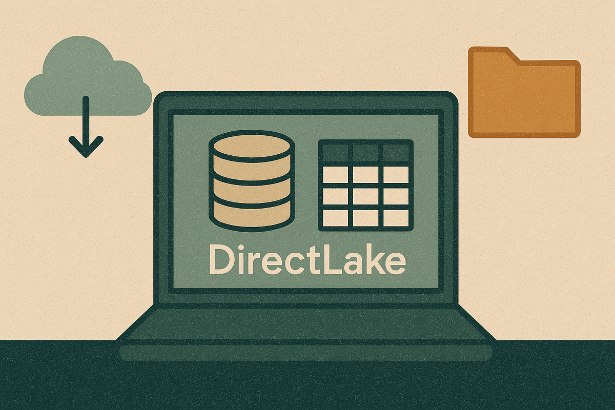
From the Gold tables, the engineer builds a Power BI semantic model using Direct Lake so reports feel “import‑fast” without nightly data copies. Direct Lake reads Delta tables in OneLake straight into memory—so coaches can slice film‑grade data interactively without waiting.

Security: Players get a personal view; coaches see their room; coordinators and the HC see the whole team. That’s row‑level security (RLS) in Power BI: filters that restrict rows per role. (Note: RLS limits apply to Viewer‑level users; workspace Admin/Member roles bypass RLS by design—your engineer will use the right roles.)

Optional live signals: If you want live stats from the sideline tablet or wearables, Fabric’s Real‑Time Intelligence can ingest streams, transform them, and light up a simple “game day board” alongside your scouting notes—then archive those events for later analysis.

Governance everywhere: Fabric’s Purview hub and Domains organize data (e.g., an Athletics domain), apply sensitivity labels, and give leadership a clear view of what’s protected and endorsed. That keeps you aligned with district expectations for student data.

What coaches get (every week and across the season)

• Team Sheet (Monday): The single pager you already use—now backed by a model you can trust for trends and drill‑down.
• Player Cards (private): Grade %, ME rate, touches/targets/havoc plays, consistency streaks, and a short list of “next reps.”
• Room Dashboards:
  • OL: pressure/sack accountability, technique flags (“late hands,” “fit late”), situational splits (3rd & medium, low red).
  • Skill: route depth consistency, decision quality, yards after contact trends.
  • Defense/ST: leverage/fit outcomes, impact plays, coverage/tackle reliability.
• Season Trends: Week‑over‑week ME rate, “win” rate by concept, opponent‑adjusted grades, class‑year cohorts, and offseason baselines that inform summer focus.

All of this stays coach‑friendly because the data engineer bakes the definitions into the semantic model once—and everyone uses the same truth thereafter.

How the partnership runs (no drama)

Your job stays the same: grade the film with the simple rubric and leave one‑phrase notes where they change practice. The apps you’re already using remain the front door.

The engineer’s steady cadence:

1. Keep the Dataverse → OneLake link healthy (automatic mirroring).
2. Maintain Silver/Gold transforms (Dataflows Gen2 or notebooks) and the star schema.
3. Evolve the Power BI model (measures you care about, like “Drive‑ending MEs”).
4. Govern access (RLS for players, workspace roles for staff, sensitivity labels in Purview).
5. Publish a Power BI app to staff and players so nobody is hunting for links.

A note on licensing (so you can plan)

• Authors/publishers (the engineer and any coach who edits reports) need Power BI Pro.
• Report consumers (read‑only viewers) typically also need Pro, unless your district licenses a Fabric capacity at F64 or higher—in which case Free viewers can access content in workspaces on that capacity. Your engineer can help align the workspace to whatever you have.

Starter scope (what we actually build first)

1. Link Dataverse to Fabric (players, games, plays, on‑field, grades mirror into OneLake).
2. Gold model with just the essentials: FactPlayerPlayGrade, DimPlayer, DimGame, DimOpponent, DimPositionGroup.
3. Power BI semantic model in Direct Lake + three reports:
   • Team Sheet (game rollups).
   • Room View (filters + technique flags).
   • Private Player Card (RLS).
4. OneLake Shortcut to any external CSV (e.g., practice attendance) to enrich Player Cards without copying data.
5. Purview basics: sensitivity labels + endorsement so admins know what’s trusted.

From there, add opponent scouting cuts, practice‑plan exports, or real‑time sideline boards as you see value.

Guardrails for student data (plain talk)

• Least privilege: players = Viewer + RLS; position coaches see only their room; coordinators/HC get team‑wide. (Admins and Members in a workspace bypass RLS—so keep those roles tight.)
• Governance: put your items in an Athletics domain; apply sensitivity labels; monitor with Purview hub. Your district data lead will appreciate the visibility.

Why Fabric + Power BI works for high school programs

• One system of record from your grading apps to your dashboards—no wobbly exports.
• Fast, coach‑friendly reports via Direct Lake (open, filter, decide).
• Zero‑copy expansion with OneLake Shortcuts when you want to fold in other files/sources.
• Built‑in governance your district already understands (Purview + domains, RLS).

If you want this as an “Athletics Analytics” blueprint, the ingredients above are all you need. Your staff keeps doing what works on Saturday; the data engineer quietly turns that into compounding advantage by Monday—and keeps the season’s trail of evidence organized for next year’s goals.

I often hear that DirectLake “removes the ability to define tables” and “doesn’t work like traditional Power BI or Tableau.” At a glance, the workflow is different—deliberately so—because Fabric is a data platform, not a visualization tool. In the old days we’d push transformations past gold and into the semantic layer because that was the only practical place left. That was necessary; it was never ideal. By definition, gold is supposed to be ready to consume.

DirectLake mode in MS Fabric’s Power BI gives you (almost) everything Power BI gave you in Desktop. The one big thing you don’t do anymore is DAX calculated columns/tables—and that’s a feature, not a bug. Nuance for accuracy: In DirectLake, calculated columns and calculated tables that reference DirectLake tables aren’t supported; however, some calculated tables that don’t reference DirectLake tables (e.g., documentation helpers) and calculation groups/what‑if parameters are allowed. DirectLake reads Delta in OneLake, the model still uses VertiPaq, and data prep moves into the platform (Dataflows Gen2, Lakehouse/Warehouse SQL, notebooks).

Turning small, theory‑driven tests into compounding results

Improvement science is simple and powerful: start with a clear theory of change, run a safe test, study the data, then adopt, adapt, or abandon. The challenge isn’t running one test—it’s running hundreds of small tests, keeping their intent and results visible, and scaling what works without losing the thread.

Microsoft Fabric is a strong fit because it lets you keep the learning system (ideas, theories, PDSA cycles, decisions) right next to the evidence system (measures and run charts). Below is a high‑level pattern that puts improvement science at the center, with examples from manufacturing and oil & gas.

I’ll be following FabConEurope closely (Sept 15–18, Austria Center Vienna) to see how the newest Microsoft Fabric capabilities land in real‑world talks and demos. Here’s the short list I’m watching—centered on near‑zero copy patterns, Materialized Lake Views, Shortcut Transformations, and Real‑Time Intelligence.

This post demonstrates Materialized Lake Views (MLVs) in a realistic Microsoft Fabric setup. We pair MLVs with Real‑Time Intelligence (RTI)—specifically an Eventhouse (KQL database)—to show how event‑scale data (lap times and race results) can feed a medallion‑style model with no bespoke pipelines and clean governance.

We’ll use the Kaggle Formula 1 World Championship dataset (link shows 1950–2024) and build this end‑to‑end:

• Eventhouse (RTI) to own lap_times and results, surfaced to OneLake as Delta via OneLake Availability.
• Lakehouse to declare MLVs (Silver/Gold) over those Delta tables.
• Warehouse to query Lakehouse tables with three‑part names (no replication).
• Power BI Semantic Model in Direct Lake over the materialized Delta outputs.

1) Concept & dataset

Concept: Make MLVs the “engine” of your medallion layers. Keep high‑volume facts in Eventhouse, expose them to OneLake as Delta, and declare your Silver/Gold logic as MLVs in the Lakehouse. Query the results from a Warehouse and publish a Direct Lake model—without wiring separate pipelines or scattering logic across tools.

Dataset: Kaggle — Formula 1 World Championship (1950–2024). You’ll use:
drivers.csv, constructors.csv, circuits.csv, races.csv, results.csv, lap_times.csv.

2) Reference architecture (MLV‑first)

Kaggle CSVs (drivers, constructors, circuits, races, results, lap_times)
        └──► Eventhouse (KQL DB): ingest CSVs as KQL tables
               └──► OneLake Availability: exposes Eventhouse tables as Delta

Lakehouse
  └──► Table Shortcuts to the Eventhouse-backed Delta tables
  └──► Materialized Lake Views (Silver/Gold) declared in Spark SQL

Warehouse (SQL)
  └──► Cross-database queries (database.schema.table) against Lakehouse Delta

Power BI
  └──► Direct Lake model bound to MLV Delta outputs (avoid SQL views to prevent fallback)

Why this pattern? Eventhouse is purpose‑built for event‑scale ingestion and ad‑hoc KQL. OneLake Availability turns those tables into Delta so every other engine can read them without copy steps. MLVskeep transformation logic declarative, governable, and monitorable.

3) Create Fabric items

• Eventhouse (KQL DB): f1_event
• Lakehouse: f1_lake (enable schemas)
• Warehouse (SQL): f1_wh (optional but useful for SQL demos)

Note that when you create your lakehouse, you won’t see a default semantic model. This model has been sunset, and now you will need to create a semantic model manually, following best practice. This avoids a number of errors.

4) Load the dataset into Eventhouse (KQL)

Use the Eventhouse ingestion wizard or KQL commands. Below is a concise pattern you can adapt.

4.1 Create tables

// Event tables
.create table lap_times (
  raceId:int, driverId:int, lap:int, position:int, [time]:string, milliseconds:long
);

.create table results (
  resultId:int, raceId:int, driverId:int, constructorId:int,
  number:int, grid:int, position:string, positionText:string, positionOrder:int,
  points:real, laps:int, [time]:string, milliseconds:long,
  fastestLap:int, rank:int, fastestLapTime:string, fastestLapSpeed:real,
  statusId:int
);

// Reference tables
.create table drivers (
  driverId:int, driverRef:string, number:int, code:string,
  forename:string, surname:string, dob:string, nationality:string, url:string
);

.create table constructors (
  constructorId:int, constructorRef:string, name:string, nationality:string, url:string
);

.create table circuits (
  circuitId:int, circuitRef:string, name:string, location:string,
  country:string, lat:real, lng:real, alt:int, url:string
);

.create table races (
  raceId:int, year:int, round:int, circuitId:int,
  name:string, [date]:string, [time]:string, url:string
);

4.2 Define CSV mappings (example for one table; repeat as needed or use the wizard)

.create table results ingestion csv mapping "ResultsCsv"
'['
 '{"column":"resultId","datatype":"int","Ordinal":"0"},'
 '{"column":"raceId","datatype":"int","Ordinal":"1"},'
 '{"column":"driverId","datatype":"int","Ordinal":"2"},'
 '{"column":"constructorId","datatype":"int","Ordinal":"3"},'
 '{"column":"number","datatype":"int","Ordinal":"4"},'
 '{"column":"grid","datatype":"int","Ordinal":"5"},'
 '{"column":"position","datatype":"string","Ordinal":"6"},'
 '{"column":"positionText","datatype":"string","Ordinal":"7"},'
 '{"column":"positionOrder","datatype":"int","Ordinal":"8"},'
 '{"column":"points","datatype":"real","Ordinal":"9"},'
 '{"column":"laps","datatype":"int","Ordinal":"10"},'
 '{"column":"time","datatype":"string","Ordinal":"11"},'
 '{"column":"milliseconds","datatype":"long","Ordinal":"12"},'
 '{"column":"fastestLap","datatype":"int","Ordinal":"13"},'
 '{"column":"rank","datatype":"int","Ordinal":"14"},'
 '{"column":"fastestLapTime","datatype":"string","Ordinal":"15"},'
 '{"column":"fastestLapSpeed","datatype":"real","Ordinal":"16"},'
 '{"column":"statusId","datatype":"int","Ordinal":"17"}'
']';

4.3 Ingest from storage

My recommendation here is to use the wizard to ingest the data you need via a shortcut. (I pulled the data for the “changeable” items, like the results and standings from an Azure Blob Storage data source after I had truncated them to remove the 2024 data so that we can demonstrate ingesting new data through the eventhouse.

1. Click on the ellipsis next to the desired table (…)
2. Click “Get Data”
3. Choose your storage method
4. Fill out your connection details (making sure to properly filter your data to only a single file format)
5. Validate your schema mappings
6. Complete!

For completeness, I also created tables for the remaining reference tables: seasons and status, which is supported from this same interface.

5) Enable OneLake Availability on Eventhouse

Turn it on at the database or table level. Eventhouse will publish the KQL tables to OneLake as Delta with a governed latency window. While enabled, some operations (e.g., rename) are restricted. This makes your data instantly consumable by Lakehouse, Warehouse, and Power BI without extra copy steps.

6) In the Lakehouse, create Table Shortcuts to Eventhouse tables

Create new schemas, bronze, silver, and gold in the lakehouse.

From f1_lake → Tables → bronze ▸ New Shortcut → Source: KQL database → select drivers, constructors, circuits, races, results, lap_times.
They appear as Delta tables in the Lakehouse—queryable by Spark, the SQL analytics endpoint, and Direct Lake.

7) Declare Materialized Lake Views (MLVs)

Prereqs: In the Lakehouse, schemas must be enabled. Create MLVs from a notebook using Spark SQL. You’ll monitor, schedule, and see lineage from the Managed materialized lake views pane.

7.1 Silver layer (standardize/enrich)

-- silver.dim_driver
CREATE MATERIALIZED LAKE VIEW IF NOT EXISTS silver.dim_driver AS
SELECT CAST(driverId AS INT)          AS driver_id,
       CONCAT(forename, ' ', surname) AS driver_name,
       code,
       nationality,
       CAST(dob AS DATE)              AS dob
FROM drivers;

-- silver.dim_constructor
CREATE MATERIALIZED LAKE VIEW IF NOT EXISTS silver.dim_constructor AS
SELECT CAST(constructorId AS INT) AS constructor_id,
       name AS constructor_name,
       nationality
FROM constructors;

-- silver.dim_circuit
CREATE MATERIALIZED LAKE VIEW IF NOT EXISTS silver.dim_circuit AS
SELECT CAST(circuitId AS INT) AS circuit_id,
       name AS circuit_name,
       location,
       country
FROM circuits;

-- silver.dim_race (join circuits)
CREATE MATERIALIZED LAKE VIEW IF NOT EXISTS silver.dim_race AS
SELECT r.raceId             AS race_id,
       r.year               AS season,
       r.round,
       r.name               AS race_name,
       CAST(r.date AS DATE) AS race_date,
       r.circuitId          AS circuit_id,
       c.circuit_name,
       c.location,
       c.country
FROM races r
LEFT JOIN silver.dim_circuit c
  ON r.circuitId = c.circuit_id;

-- silver.results_clean with data quality
CREATE MATERIALIZED LAKE VIEW IF NOT EXISTS silver.results_clean
(
  CONSTRAINT pos_order_valid CHECK (positionOrder >= 1) ON MISMATCH DROP,
  CONSTRAINT points_nonneg   CHECK (points >= 0)        ON MISMATCH FAIL
)
AS
SELECT resultId, raceId, driverId, constructorId,
       grid, positionOrder, points, laps,
       fastestLap, fastestLapTime, fastestLapSpeed
FROM results;

-- (Optional) silver.laps_clean
CREATE MATERIALIZED LAKE VIEW IF NOT EXISTS silver.laps_clean
(
  CONSTRAINT lap_ms_nonneg CHECK (milliseconds >= 0) ON MISMATCH DROP
)
AS
SELECT raceId, driverId, lap, position, milliseconds
FROM lap_times;

7.2 Gold layer (analytics‑ready facts)

-- gold.fact_results
CREATE MATERIALIZED LAKE VIEW IF NOT EXISTS gold.fact_results AS
SELECT d.driver_id,
       co.constructor_id,
       r.season,
       r.race_id,
       rc.grid,
       rc.positionOrder AS finish_pos,
       rc.points,
       rc.laps,
       rc.fastestLap,
       rc.fastestLapTime,
       rc.fastestLapSpeed
FROM silver.results_clean rc
JOIN silver.dim_race       r  ON rc.raceId       = r.race_id
JOIN silver.dim_driver     d  ON rc.driverId     = d.driver_id
JOIN silver.dim_constructor co ON rc.constructorId = co.constructor_id;

-- gold.fact_laps
CREATE MATERIALIZED LAKE VIEW IF NOT EXISTS gold.fact_laps AS
SELECT r.season,
       l.raceId       AS race_id,
       l.driverId     AS driver_id,
       l.lap,
       l.position     AS lap_position,
       l.milliseconds AS lap_time_ms
FROM silver.laps_clean l
JOIN silver.dim_race  r ON l.raceId = r.race_id;

Operate the MLVs: From Manage materialized lake views, set a schedule, trigger a manual refresh, review lineage, and inspect data‑quality results (dropped rows vs. failures). Current behavior is full refresh on change; runs are skipped when no inputs changed.

8) Query from the Warehouse (no copies)

From f1_wh, use three‑part names (database.schema.table) to query Lakehouse tables directly:

-- Inspect gold fact
SELECT TOP 10 *
FROM f1_lake.gold.fact_results
ORDER BY season DESC, race_id DESC;

-- Top winners
SELECT d.driver_name, COUNT(*) AS wins
FROM f1_lake.gold.fact_results fr
JOIN f1_lake.silver.dim_driver d
  ON fr.driver_id = d.driver_id
WHERE fr.finish_pos = 1
GROUP BY d.driver_name
ORDER BY wins DESC;

9) Build the Semantic Model (Power BI) in Direct Lake

Bind model tables directly to the Delta outputs (gold.*, selected silver.*). Avoid layering SQL views between Power BI and your Delta tables; views can cause Direct Lake → DirectQuery fallback. Use physical Delta tables (your MLV outputs) for the best performance.

Starter DAX

Wins := COUNTROWS( FILTER( 'fact_results', 'fact_results'[finish_pos] = 1 ) )
Podiums := COUNTROWS( FILTER( 'fact_results', 'fact_results'[finish_pos] <= 3 ) )
Avg Lap (ms) := AVERAGE('fact_laps'[lap_time_ms])
Points := SUM('fact_results'[points])

10) Notes & gotchas

• MLVs today: created via Spark SQL; refresh is full on change with skipped runs when unchanged.
• Eventhouse availability: while enabled, certain DDL operations (e.g., rename) are restricted; configure latency to balance freshness vs. cost.
• Direct Lake: binding to tables (not SQL views) avoids fallback to DirectQuery.
• Alternate path for reference data: If you prefer not to store dims in Eventhouse, you can import the CSVs into the Lakehouse as Delta (e.g., “Create table from files” or a short Spark notebook). This does create a managed copy, but keeps your MLV story intact—still no separate pipeline tool required.

11) Quick validation

KQL (Eventhouse)

results
| summarize total_points = sum(points) by driverId
| top 10 by total_points desc

Spark SQL (Lakehouse)

SELECT season, COUNT(DISTINCT race_id) AS races
FROM gold.fact_results
GROUP BY season
ORDER BY season DESC;

T‑SQL (Warehouse)

SELECT TOP 20 r.season, r.race_name, d.driver_name, fr.finish_pos, fr.points
FROM f1_lake.gold.fact_results AS fr
JOIN f1_lake.silver.dim_race   AS r ON fr.race_id   = r.race_id
JOIN f1_lake.silver.dim_driver AS d ON fr.driver_id = d.driver_id
ORDER BY r.season DESC, r.race_id DESC, fr.finish_pos ASC;

Why Materialized Lake Views (MLVs) matter

• Declarative pipelines: one Spark SQL statement defines each transform. Fabric handles orchestration, lineage, and monitoring—no separate ETL/pipeline asset to wire up.
• Governed & observable: MLVs show source dependencies, run history, and data‑quality outcomes in a single, first‑class UI.
• Built‑in data quality: add CHECK constraints with ON MISMATCH DROP | FAIL to reject or fail on bad data—without custom code.
• Predictable refresh: full refresh when sources change, skipped runs when they don’t—simple behavior that’s easy to explain to stakeholders.
• Open downstream: MLV outputs are Delta tables in OneLake—query them from Warehouse (SQL), notebooks, and Power BI in Direct Lake for fast BI.

Closing

MLVs turn your medallion layers into governed assets: one statement per transform, first‑class lineage, schedulable refresh, and built‑in data quality. Pair them with Eventhouse and OneLake Availability to keep ingestion fast and analytics open—then light up Warehouse and Direct Lake without extra copy steps or pipeline sprawl.